The purpose of this section is to demonstrate the connection process for specific pieces of equipment. This is less so a tutorial on how to use different code interfaces, and more about how we connect to the hardware in the first place. This section will describe the required python packages, external software, and source code edits necessary to connect to instruments. In nearly every circumstance, this initial connection is then wrapped by a new python class which provides slightly more convenient functions that can then interface with the rest of the package. Look out for the “Making the Connection” tips that describe the requirements for using each specific instrument!
Alicat MFCs
Note
The Alicat Python package was updated with a breaking change after implementation into the Catalight project. Version 0.4.1 is the last compatible version and has been hard pinned into the Catalight requirements file.
Alicat brand MFCs are accessed utilizing the Alicat python package developed by Patrick Fuller and Numat.
For proper gas monitoring, many mass flow controllers need to be supplied with the appropriate process gas composition. Alicat flow controllers are capable of creating custom gas mixtures comprised of some combination of the gas library hosted by the device. This feature is implemented in the gas_system class of catalight for creating calibration gasses, and output gas compositions when using a flow meters after gas mixing. The following links provide additional information for Alicat systems:
Warning
This automated gas system has no ability to check gas mixing safety! It is your responsibility to ensure chemical compatibility before mixing gasses. Always check for leaks and ensure the system is free of pressure build ups before leaving the system unattended or flowing hazardous gasses.
Making the Connection
As of v0.2.0, the COM ports for the individual MFC addresses are defined by the config.py file. New users need to edit these addresses in a forked version of the source code for successful connection. At the moment, the MFC count is hard coded for 4 MFCs and one output flow meter at the moment, and significant code changes to the source code are needed to change the MFC count. This will soon be updated such that the user only has to specify the number of MFCs in the config file. The catalight.equipment.alicat_connection_tester module can be used to aid in determining the MFC COM ports. If can be helpful to change the MFC address (A, B, C, etc) directly on the hardware prior to trying to interface through catalight. See Areas for Future Development for more details. Additional software shouldn’t be necessary.
Harrick Heater/Watlow
The Harrick reaction chamber’s heating system is controlled by a Watlow temperature controller. In place of using the EZ-ZONE configurator software, we utilize the pywatlow package developed by Brendan Sweeny and Joe Reckwalder. Brendan has an excellent write up describing the creation of the project. Our Heater class simply add some additional utilities on top of the pywatlow project, such as unit conversions, and ramped heating. In theory, the Heater class should work with any Watlow controlled heater, but we have only tested it with the Harrick system. Note that Harrick provides a calibration file for this equipment which should be installed using the EZ zone configurator. We have not confirmed that these calibrations port over succesfully into the the Heater class.
Tip
Other parameters are accessible using pywatlow. See the “Operations” section of the manual located in the catalight/equipment/harrick_watlow directory.
Making the Connection
The COM ports for the Watlow heater are are defined by the config.py file. New users need to edit these addresses in a forked version of the source code for successful connection. Additional software should not be needed, though testing your connection with the EZ zone configurator software can be helpful for troubleshooting, and calibration.
ThorLabs Laser Diode Driver
Warning
Lasers present serious safety hazards, even in lab environments. This is especially true when software is used to automatically control them. Always take abundant safety precautions to ensure laser beams are physically contained. Never assume the code is working properly. Don’t rely on the software to turn the laser off and assume you can enter the laser lab without safety glasses on. Always be in the room when engaging the laser via code, and always use safety interlocks and message boards to alert other users that an unattended laser is active.
We use the LDC200C Series Laser Diode Driver to control our diode laser excitation source. The driver does not have a computer interface, but supports current modulation via a 10 Volt analog signal supplied by a BNC connection at the rear of the device. To supply an analog signal to the current controller, we utilize a USB-231 DAQ card from Measurment Computing Corporation (MCC). MCC publishes a Python API for their Universal Library (mcculw). We also utilize their instacal software for installing the DAQ and setting the board number, though this may not be strictly necessary when using the mcculw library. Our Diode_Laser class hides interaction with the mcculw from the user, favoring method calls such as “Diode_Laser.set_power()” over interacting directly with the DAQ board. The intention is to ignore the existence of the DAQ interface when operating the laser programmatically. In fact, this makes some troubleshooting activities a bit easier for the Diode_Laser class as the laser can remain off (by unplugging or pressing the physical off switch) while the user interacts safely with the DAQ board. All commands will remain functional, though voltage readings from the current driver output won’t return realistic values.
In version 1 of Catalight, the diode laser class relies on a auxiliary script to perform calibraiton (unlike the NKT_System which has calibration as a built in method). This was originally done because the calibration needs to be performed in conjunction with a power meter. More information about performing the calibration can be found in the section: Laser calibration
Making the Connection
It isn’t completely necessary to install additional software before using a Diode_Laser instance, but you will need to install the MCC DAQ board in some way. We suggest you install and use instacal, but there is a command line method documented in the mcculw library
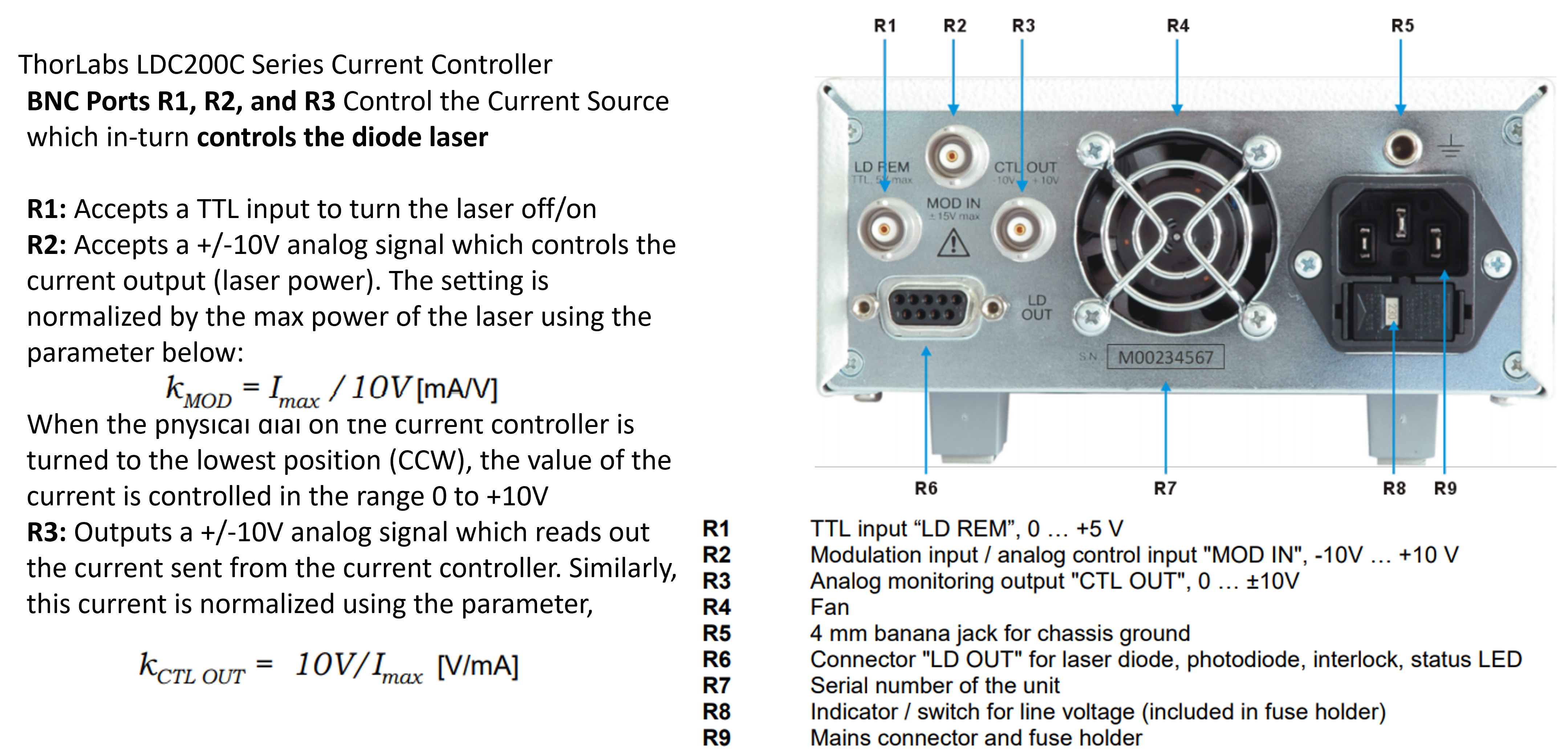
Screenshot from Thorlabs current driver manual showing where BNC connections need to be made along with the voltage to current conversion factors used. Note that these values may need to change if you have a different model number!
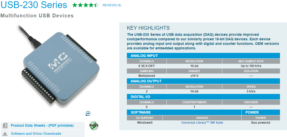
Screenshot of product page for the DAQ board used in D-Lab hardware configuration
NKT Fianium/Extreme + Varia System
Warning
Lasers present serious safety hazards, even in lab environments. This is especially true when software is used to automatically control them. Always take abundant safety precautions to ensure laser beams are physically contained. Never assume the code is working properly. Don’t rely on the software to turn the laser off and assume you can enter the laser lab without safety glasses on. Always be in the room when engaging the laser via code, and always use safety interlocks and message boards to alert other users that an unattended laser is active.
Support for an NKT laser and the Varia tunable emission system is provided through the catalight.equipment.light_sources.nkt_system.NKT_System class. The NKT connection is acheived through NKT’s DLL interface. To simplify the interaction with the user, we developed this interface as a seperate python package, nkt_tools, which is installed as a requirement of the catalight package. The DLL file is also included in the source files of nkt_tools, so no additional software should be needed to interface with the NKT system.
The nkt_tools package provides a python interface for the NKT Varia and Extreme/Fianium individual, whereas the NKT_System class bundles the Varia and laser into a single interface. In the first iteration of this tool (v0.2.0), the hardware is configured without an inline power meter and power management is handled by varying the power setpoint (in %) of the Fianium/Extreme. This type of power management alters the output spectrum of the laser, making the power output (in mW) non-linear. We try to circumvent this challenge by performing a calibration on the system (described below), but future users should consider utilizing a computer controlled neutral density filter or incorporating an inline power meter to monitor the NKT output. In the former case, the NKT could be set to 100% power output, and the delivered power (in mW) could be more easily calibrated since the output spectrum shouldn’t change with an ND filter. In the latter case, a certain percent of the NKT laser could be monitored to inform the software of the delivered power, and a feedback loop can be written to better deliver the requested power.
Making the Connection
All of the connection needed for the NKT System should be handled automatically, and the user should only need to plug in their system to the computer. It is necessary to calibrate the NKT system prior to use.
Calibrating the NKT_System:
The NKT_System provides a calibration prodedure utilizing the method run_calibration(). An example script for running the calibration process is provided below. Note, the calibration process takes a few hours to complete.
from catalight.equipment.light_sources import nkt_system
from catalight.equipment.power_meter import newport


meter = newport.NewportMeter()
nkt = nkt_system.NKT_System()

nkt.run_calibration(meter)
The strategy of the calibration process is to vary the central wavelength of the NKT Varia and compute the spectrally averaged power output for each central wavelength. This is done using a bandwidth of 10 nm, moved in increments of 1 nm. The spectral power density is computed as a mW/nm value, and this process is repeated for multiple power setpoints (in percents). The outcome of the calibration process is seen below:

Calculated spectral power of laser based on wavelength sweeps at various setpoints.
The raw data is fit on a power setpoint vs power output function for each wavelength value tested, as shown in the figure below. Especially for short wavelengths, the fit function is non-linear.

Compilation of fits for select wavelengths across different power settings. The top left value in each subplot indicates the last wavelength plotted, givin an approximate wavelength range for each plot.
An algorithm is used to compute the expected laser output for a given laser setpoint value under a given set of optical conditions (central wavelength and bandwidth). Several benchmarking tests are performed in the course of the calibration process to check the accuracy of the calibration. A measurement is performed by setting a fixed short pass value and extending the bandwidth out from the min to max bandwidth value. The predicted vs measured output values are compared so that the user can get a sense for the error of the calibration performance. Similarly, the calibration data itself is plotted as a “growing window” test in which a 10 nm bandwidth window is moved across the spectrum. The power output by a given setpoint value is computed and the error is plotted in terms of (LHS) what power is expected vs measured and the (RHS) what power setpoint should be needed to acheive the measured power output. In this sense, the calibration formula is being solved in “both directions”
In all benchmarking cases, no verifications are performed by the software. The user must manually evaluate the performance of the system and judge whether the performance is acceptable.

Predicted and measured powers output by the laser for a variable bandwidth showing the error associated with changing the bandwidth feature.

Predicted power and measured power for a moving window test. A fixed bandwidth is moved across the laser spectrum, and the requested power is compared to the measured value.
Finally, the calibration is verified using a randomized comparison. Random power outputs, center wavelengths, and bandwidths are requested from the system. If the optical conditions are acheivable (the power is within the measured limits) then the system actuates those conditions and measures the output power. The results are plotted as a function of the requested output power, but the data points also differ in central wavelength and bandwidth to give a more varied few of the calibration performance. On the Dionne Lab system, there is a constant over estimate of the output power causing slightly lower power output than requested.

Predicted power vs measured power for randomized optical conditions, post-calibration.
It should be noted that there is a significant error in the power output produced in this manner. I would suggest that users establishing a new experimental setup consider placing a power meter permanently in-line with the system using a beam splitter such that a fraction of the power output is always being measured. The calibration process is slow, tedious, and inaccurate.
Power meter
A power meter is programmatically controlled in order to run laser power calibrations. We currently use the Newport 843-R-USB accessed via Newports' PMManager's COM object. This method should also allow the user to control the 1919-R, 843-R-USB , 844-PE-USB , 845-PE-RS, 1938-R, and 2938-R models with no additional changes, but these models have not been tested. Additional commands could be accessed via the provided COM object if desired. See the user commands manual for more information.
Making the Connection
A version of Newport’s PMManager COM object is required and needs to be installed in order to use the NewportMeter class. This can be installed from https://www.newport.com/t/PMManager-power-meter-application-software. Installing the full PMManager software includes the COM object, and no additional code changes should be needed after the installation.
SRI Gas chromatograph
In our lab, we use the 8610C MULTIPLE GAS ANALYZER #5 GC from SRI instruments with an FID and TCD detector. There is no python package available to control SRI GCs as far as we know (2023/02/16). However, SRI provides a remote control interface in the form of an “API provided through a .NET assembly”. This is downloaded when you install a version of peaksimple onto your lab computer within a zip file called PeaksimpleConnectorTestClient.zip. We include an unzipped version of this package within the catalight/equipment/gc_control directory. The end-user does not need to install PeaksimpleConnector files, but will need an instance of peaksimple installed on the computer. The official documentation file from the SRI website is also stored in this directory as PeakSimpleRemoteControlJune2014.pdf if a user would like to see more information about SRI’s API.
What does this mean and what is a “.NET assembly”? Essentially, .NET is a way of writing code that makes it accessible across multiple languages. Tools can be built using Visual Basic or C then accessed elsewhere in a different language through the “Common Language Runtime” so long as they are built using .NET principles. For us, this means we can access the SRI API by loading it into python with a package called python.NET. This interface works a bit differently from the other tools in this package, like those for controlling MFCs and the Watlow heater, because the API connects us to peaksimple, the GC’s software, rather than directly connecting us to the instrument. In practice, this means that an instance of peaksimple must be installed and running whenever python calls to the instrument are made.
Note
- There is a documented bug in SRI’s “PeakSimpleRemoteControlJune2014” instructions stating that
“Once a connection has been broken by stopping either Peaksimple or the calling program, the other must be restarted also before another connection can be made.”
This means that Peaksimple must be manually closed and reopened each time the catalight GUI or scripted interface is closed. If you are using this package with an interactive python kernel, you may also have to restart the kernel before reconnecting to peaksimple. The catalight GUI will attempt to open Peaksimple automatically if it isn’t already, but the user must close Peaksimple after closing the catalight GUI.
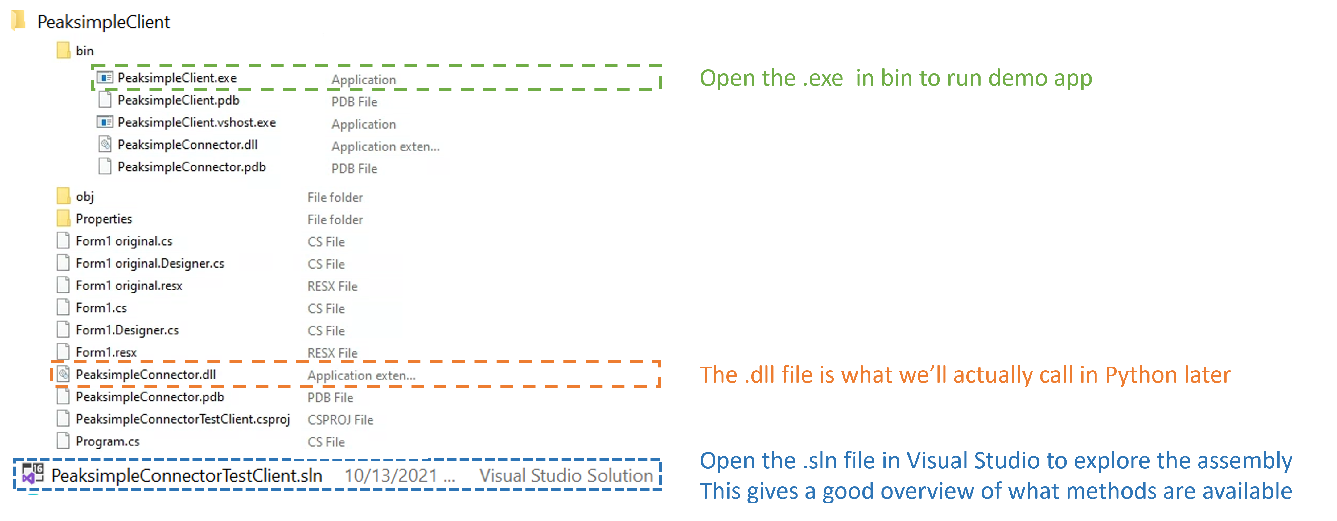
The contents of the PeaksimpleClient folder installed with Peaksimple. The three most important files are highlighted.
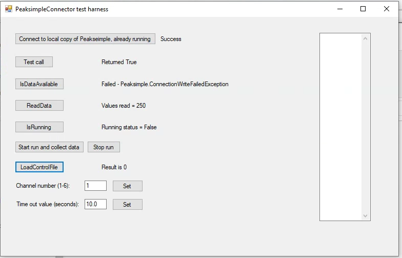
Running PeaksimpleClient.exe
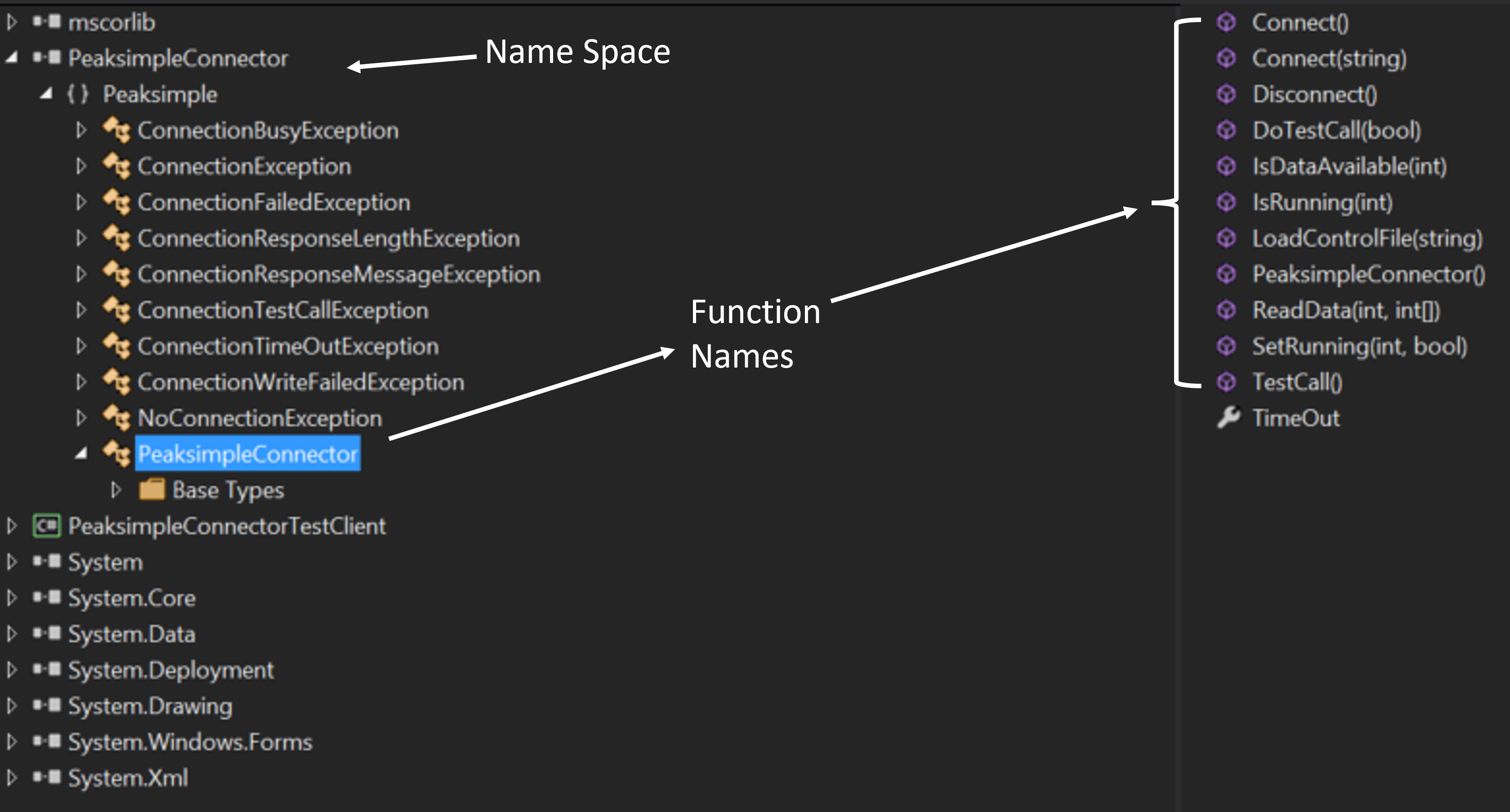
PeaksimpleConnectorTestClient.sln file contents from Visual Studio
Now that we understand the files inside of SRI’s automation toolkit, lets look at how we can import these tools into python. This is accomplished utilizing the python.NET package, which gives us access to every method you see within the PeaksimpleConnector.TestClient.sln file above.
import os
import clr  # Essentially python.NET
dir_path = os.path.dirname(os.path.realpath(__file__))
assemblydir = os.path.join(dir_path, 'PeaksimpleClient', 'PeaksimpleConnector.dll')

clr.AddReference(assmblydir) # Add the assembly to python.NET
# Now that the assembly has been added to python.NET,
# it can be imported like a normal module
import Peaksimple  # Import the assembly namespace, which has a different name
Connector = Peaksimple.PeaksimpleConnector()  # This class has all the functions

Connector.Connect() # Connect to running instance of peaksimple using class method
Connector.LoadControlFile(ctrl_file)  # Load ctrl file using class method
That pretty much gives you complete control over the GC. Notice that there are not a ton of attributes or methods within the PeaksimpleConnector class. The main interaction the user has with the equipment is achieved by editing the control files. Through editing the control file, the user can change many definitions that would usually be controlled by the peaksimple GUI, but programmatically. Most importantly, you can now set the filename, save location, number of repeats, and use Connector.SetRunning() to start connection. These interactions get wrapped for the user in the GC_Connector() class. See Examples for details on using the class.

The abbreviated contents of the .CON files, which you can open in a text editor. We edit key lines with the GC_Connector() class, which is the same as clicking check boxes and buttons in the editing window used by Peaksimple itself.
Making the Connection
You shouldn’t need to change source code to connect with an SRI GC, but you will need to download Peaksimple from SRI’s website and open the program before launching GC_Connector()